Working with Multiple Modification Types
Source:vignettes/multiple-modification-types.Rmd
multiple-modification-types.RmdIntroduction
Bacterial genomes frequently carry multiple simultaneous DNA methylation marks:
- 6mA (N6-methyladenine) — deposited by Dam methyltransferase at GATC motifs; functions in mismatch repair and cell-cycle regulation.
- 5mC (5-methylcytosine) — deposited by Dcm methyltransferase at CCWGG motifs; roles in gene regulation are less well characterized in bacteria.
- 4mC (N4-methylcytosine) — deposited by restriction-modification systems at various sequence motifs; protects against foreign DNA.
comma stores all modification types in a single
commaData object, enabling joint analysis, comparison, and
visualization across modification types.
This vignette demonstrates multi-modification workflows using the
built-in comma_example_data dataset, which contains both
6mA and 5mC sites.
Exploring Multiple Modification Types
What modifications are present?
modTypes(comma_example_data)
#> [1] "5mC" "6mA"Per-modification methylation summary
methylomeSummary() reports stats per sample. Combine it
with mod_type filtering to compare distributions:
methylomeSummary(comma_example_data, mod_type = "6mA")[,
    c("sample_name", "condition", "mean_beta", "median_beta", "n_covered")]
#>   sample_name condition mean_beta median_beta n_covered
#> 1      ctrl_1   control 0.8986871   0.9125938       200
#> 2      ctrl_2   control 0.9002143   0.9190209       200
#> 3      ctrl_3   control 0.9090365   0.9175266       200
#> 4     treat_1 treatment 0.8189668   0.9083821       200
#> 5     treat_2 treatment 0.8187088   0.9017345       200
#> 6     treat_3 treatment 0.8001237   0.9002514       200
methylomeSummary(comma_example_data, mod_type = "5mC")[,
    c("sample_name", "condition", "mean_beta", "median_beta", "n_covered")]
#>   sample_name condition mean_beta median_beta n_covered
#> 1      ctrl_1   control 0.8062786   0.8269522       100
#> 2      ctrl_2   control 0.8180777   0.8349952       100
#> 3      ctrl_3   control 0.8163698   0.8259261       100
#> 4     treat_1 treatment 0.8027020   0.8091425       100
#> 5     treat_2 treatment 0.8035412   0.8313988       100
#> 6     treat_3 treatment 0.8012519   0.8174652       100
Distribution Comparison Across Modification Types
plot_methylation_distribution() automatically facets by
modification type when multiple types are present:
plot_methylation_distribution(comma_example_data, per_sample = TRUE)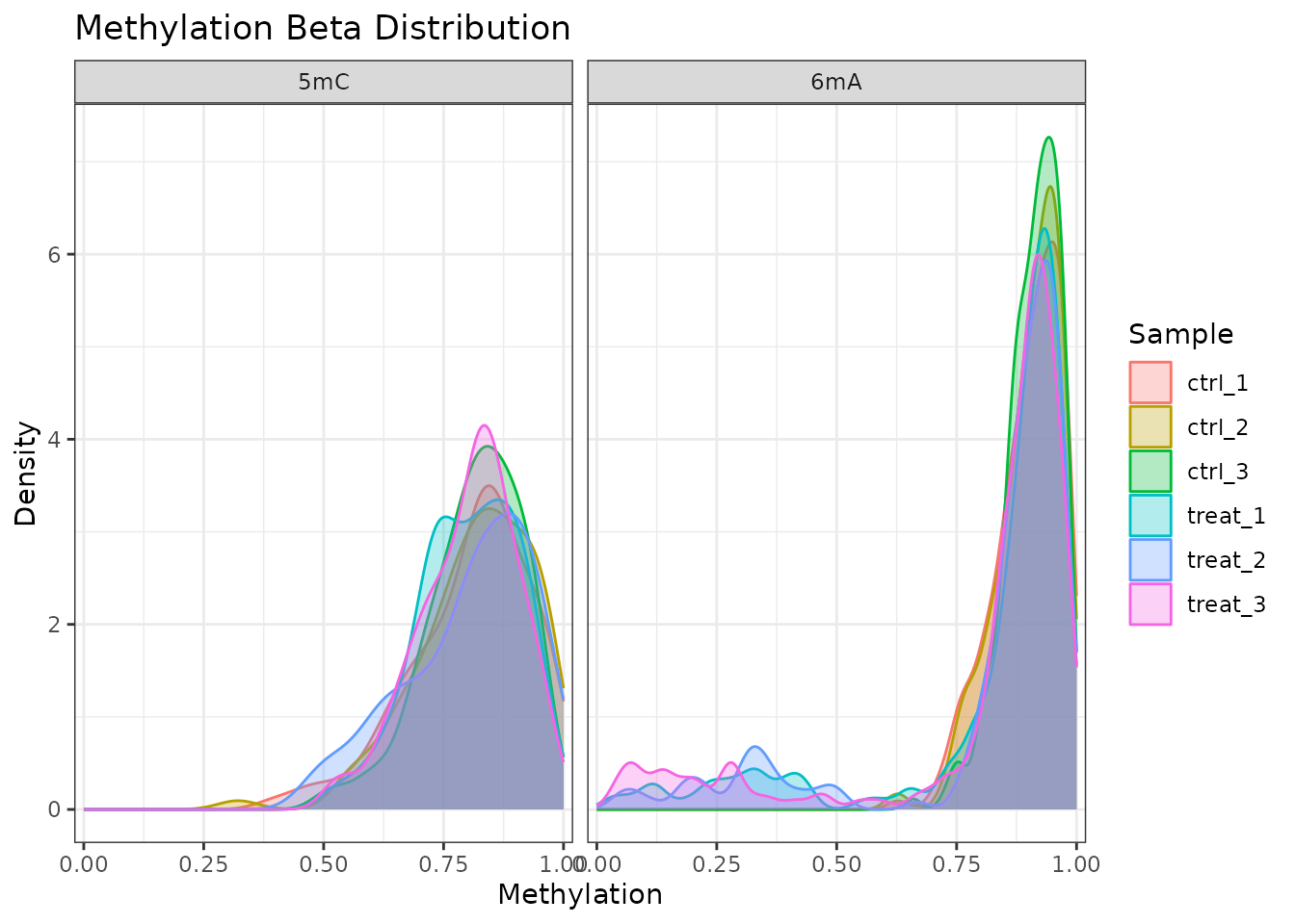
Beta value density per sample, faceted by modification type.
6mA sites in bacteria commonly show a bimodal distribution (near 0 or near 1) because restriction-modification systems methylate recognition sequences with high efficiency. 5mC patterns can be more variable.
Subsetting by Modification Type
Use subset() to extract a single modification type:
only_6ma <- subset(comma_example_data, mod_type = "6mA")
only_5mc <- subset(comma_example_data, mod_type = "5mC")

cat("6mA sites:", nrow(methylation(only_6ma)), "\n")
#> 6mA sites: 200
cat("5mC sites:", nrow(methylation(only_5mc)), "\n")
#> 5mC sites: 100
Differential Methylation: Testing Each Modification Type
Test all types in one call
By default, diffMethyl() tests all modification types
present in the object. Use results(..., mod_type = "6mA")
to extract type-specific results:
dm_all <- diffMethyl(comma_example_data, formula = ~ condition)
res_6ma <- results(dm_all, mod_type = "6mA")
res_5mc <- results(dm_all, mod_type = "5mC")

cat("6mA: significant sites (padj < 0.05, |Δβ| ≥ 0.2):",
    sum(!is.na(res_6ma$dm_padj) & res_6ma$dm_padj < 0.05 &
        abs(res_6ma$dm_delta_beta) >= 0.2, na.rm = TRUE), "\n")
#> 6mA: significant sites (padj < 0.05, |Δβ| ≥ 0.2): 6
cat("5mC: significant sites (padj < 0.05, |Δβ| ≥ 0.2):",
    sum(!is.na(res_5mc$dm_padj) & res_5mc$dm_padj < 0.05 &
        abs(res_5mc$dm_delta_beta) >= 0.2, na.rm = TRUE), "\n")
#> 5mC: significant sites (padj < 0.05, |Δβ| ≥ 0.2): 1
Volcano plots per modification type
p_6ma <- plot_volcano(res_6ma) +
    ggplot2::ggtitle("6mA differential methylation")
p_5mc <- plot_volcano(res_5mc) +
    ggplot2::ggtitle("5mC differential methylation")

# Arrange side by side if patchwork is available
if (requireNamespace("patchwork", quietly = TRUE)) {
    patchwork::wrap_plots(p_6ma, p_5mc, ncol = 1L)
} else {
    print(p_6ma)
    print(p_5mc)
}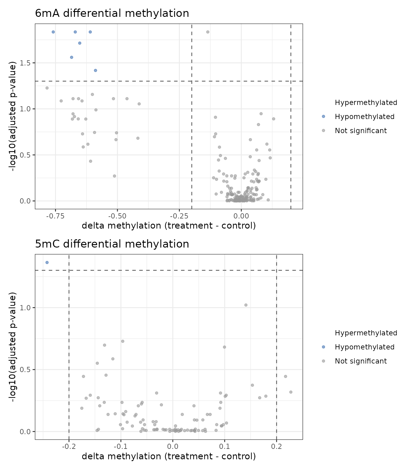
6mA differential methylation (top) and 5mC (bottom).
PCA Across Modification Types
The PCA plot uses all sites by default. Use mod_type to
restrict to a single modification type:
plot_pca(comma_example_data, color_by = "condition")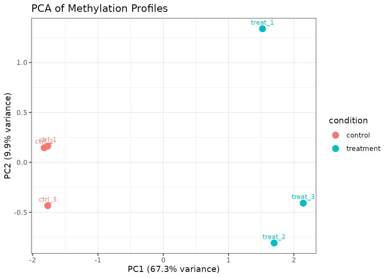
PCA using all modification types.
plot_pca(comma_example_data, mod_type = "6mA", color_by = "condition")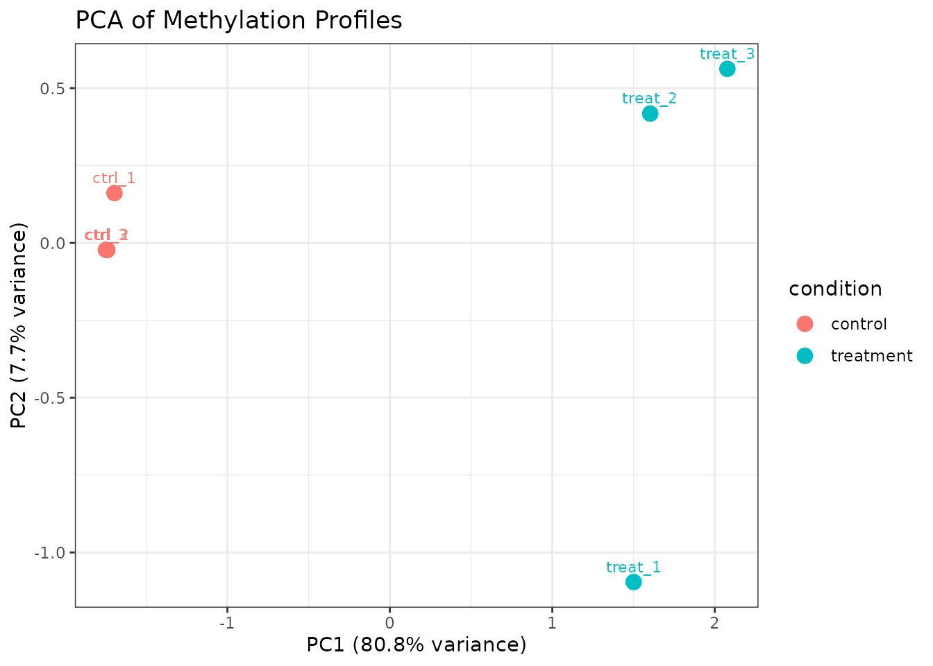
PCA using 6mA sites only.
Genome Track with Both Modification Types
When mod_type = NULL, plot_genome_track()
displays sites from all modification types, using different colors to
distinguish them:
plot_genome_track(comma_example_data, chromosome = "chr_sim",
                  start = 1L, end = 30000L, annotation = FALSE)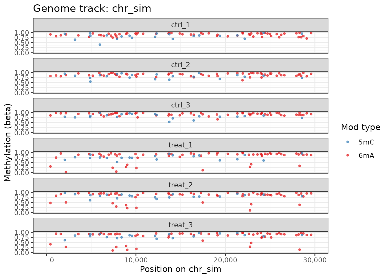
Genome track showing 6mA (red) and 5mC (blue) sites.
Heatmaps per Modification Type
Filter the results() output to a single modification
type before passing it to plot_heatmap():
plot_heatmap(res_6ma, dm_all, n_sites = 20L)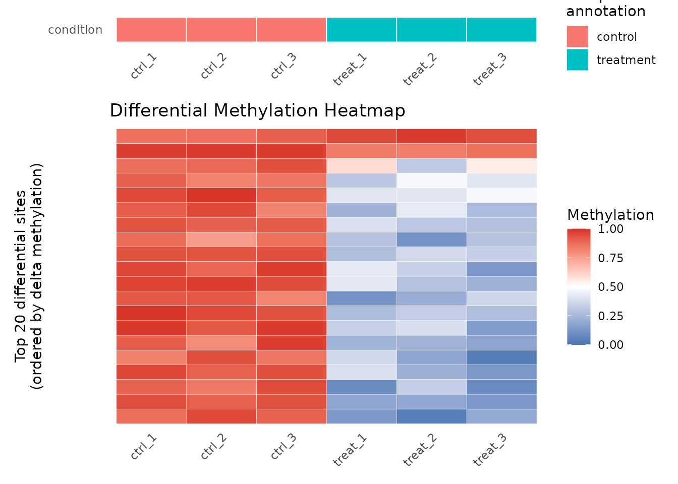
Heatmap of top 20 differentially methylated 6mA sites.
Session Information
sessionInfo()
#> R version 4.5.3 (2026-03-11)
#> Platform: x86_64-pc-linux-gnu
#> Running under: Ubuntu 24.04.3 LTS
#>
#> Matrix products: default
#> BLAS:   /usr/lib/x86_64-linux-gnu/openblas-pthread/libblas.so.3
#> LAPACK: /usr/lib/x86_64-linux-gnu/openblas-pthread/libopenblasp-r0.3.26.so;  LAPACK version 3.12.0
#>
#> locale:
#>  [1] LC_CTYPE=C.UTF-8       LC_NUMERIC=C           LC_TIME=C.UTF-8
#>  [4] LC_COLLATE=C.UTF-8     LC_MONETARY=C.UTF-8    LC_MESSAGES=C.UTF-8
#>  [7] LC_PAPER=C.UTF-8       LC_NAME=C              LC_ADDRESS=C
#> [10] LC_TELEPHONE=C         LC_MEASUREMENT=C.UTF-8 LC_IDENTIFICATION=C
#>
#> time zone: UTC
#> tzcode source: system (glibc)
#>
#> attached base packages:
#> [1] stats     graphics  grDevices datasets  utils     methods   base
#>
#> other attached packages:
#> [1] comma_0.7.1.9000 BiocStyle_2.38.0
#>
#> loaded via a namespace (and not attached):
#>  [1] SummarizedExperiment_1.40.0 gtable_0.3.6
#>  [3] xfun_0.57                   bslib_0.10.0
#>  [5] ggplot2_4.0.2               Biobase_2.70.0
#>  [7] lattice_0.22-9              vctrs_0.7.2
#>  [9] tools_4.5.3                 bitops_1.0-9
#> [11] generics_0.1.4              stats4_4.5.3
#> [13] parallel_4.5.3              Matrix_1.7-4
#> [15] RColorBrewer_1.1-3          S7_0.2.1
#> [17] desc_1.4.3                  S4Vectors_0.48.0
#> [19] lifecycle_1.0.5             compiler_4.5.3
#> [21] farver_2.1.2                Rsamtools_2.26.0
#> [23] textshaping_1.0.5           Biostrings_2.78.0
#> [25] Seqinfo_1.0.0               codetools_0.2-20
#> [27] GenomeInfoDb_1.46.2         htmltools_0.5.9
#> [29] sass_0.4.10                 yaml_2.3.12
#> [31] pkgdown_2.2.0               crayon_1.5.3
#> [33] jquerylib_0.1.4             BiocParallel_1.44.0
#> [35] DelayedArray_0.36.0         cachem_1.1.0
#> [37] abind_1.4-8                 digest_0.6.39
#> [39] bookdown_0.46               labeling_0.4.3
#> [41] fastmap_1.2.0               grid_4.5.3
#> [43] cli_3.6.5                   SparseArray_1.10.9
#> [45] patchwork_1.3.2             S4Arrays_1.10.1
#> [47] withr_3.0.2                 UCSC.utils_1.6.1
#> [49] scales_1.4.0                rmarkdown_2.30
#> [51] XVector_0.50.0              httr_1.4.8
#> [53] matrixStats_1.5.0           ragg_1.5.2
#> [55] zoo_1.8-15                  evaluate_1.0.5
#> [57] knitr_1.51                  GenomicRanges_1.62.1
#> [59] IRanges_2.44.0              rlang_1.1.7
#> [61] glue_1.8.0                  BiocManager_1.30.27
#> [63] renv_1.1.8                  BiocGenerics_0.56.0
#> [65] jsonlite_2.0.0              R6_2.6.1
#> [67] MatrixGenerics_1.22.0       systemfonts_1.3.2
#> [69] fs_2.0.1